Migrating to my school domain

I decided to move my blog to my school domain. Here is the link:

The contents of this blog will not be deleted for a while, but I also won’t be updating it. (Not that I have been updating it often.) One main advantage of moving out from WordPress is that I can now do a lot of customization; I can insert whatever code I want without any censorship. On the other hand, I need to make sure I have a host for my website, which hopefully won’t be a problem.

Eliminating aperiodicity in tilings

October 2, 2018October 2, 2018 Dongryul Kim2 Comments

This is a talk given on October 2nd, 2018, for the Harvard Math Table. I’ve been meaning to write a post on this subject, since I have been working on this problem for quite a long time now, but I never had a chance.

1. Aperiodic tilings

What are tilings? Imagine you’re an architect, and suppose you want to build your own bathroom. I’m not an architect, so I googled “how to build a bathroom”, and there was this webpage with a ${12}$ -step instruction. And three of the steps were “tile the floor”, “tile the shower”, “tile the backsplash”. Apparently, if you tile the floor and walls with ceramic tiles, they becomes more water-resistant, durable, and also attract less dust. So even if you don’t want to follow the instructions, it’s probably a good idea to tile.

There are some obvious restrictions to your plan. You don’t want there to be any part of the floor that is not covered by the tiles, and of course two tiles cannot have an overlap. Maybe you also want that there are only finitely many shapes a tile can take, to make the manufacturing process easier. We can try and formulate this as a mathematical problem.

Definition 1. A tiling of ${\mathbb{R}^2}$ is a way of covering the entire plane without overlaps by

a finite set ${S = \{ V_1, \ldots, V_n \}}$ of shapes,
and allowing translations and rotations and reflections.

More generally, we can speak of tilings of ${\mathbb{R}^d}$ for any dimension ${d}$ .

Continue reading “Eliminating aperiodicity in tilings” →

A rough guide to linear algebra

August 27, 2018 Dongryul Kim2 Comments

Around last December, I embarked on a project of writing an introductory linear algebra textbook, starting from the definition of vector spaces and leading up to the spectral theorem. Currently I have a draft that is about 150 pages long, and I plan on improving it when I have time. The book will be available for free from the following link: A rough guide to linear algebra.

The motivation for the project was a sort of academic elitism. I wanted there to be a book that would be most useful for a student with a strong mathematical background, planning to pursue a career in pure mathematics. The philosophy is very similar to that of Math 55, although I wanted to only focus on developing the theory in an abstract, morally correct manner, rather than to introduce the reader to a variety of topics.

It strikes me as peculiar that there seems to be a universal agreement among mathematicians on what the “correct abstract viewpoint of linear algebra” is, but it is difficult to find a textbook that actually develops linear algebra from this perspective. I asked myself how I learned the abstract viewpoint, but I don’t exactly remember. I guess I partly learned it from Math 55a, and later filled in the gaps by learning other mathematics such as homological algebra or vector bundles or representation theory. Well, that is not too bad a way to learn linear algebra, but I believe it is more efficient to learn linearly algebra correctly before going on to learn more advanced mathematics. For instance, it’s probably is not a good idea to learn about vector bundles before knowing why a vector space is not the same thing as its dual vector space. Continue reading “A rough guide to linear algebra” →

Maxwell’s equations

August 23, 2018August 23, 2018 Dongryul KimLeave a comment

I learned this while talking to a physics friend. It is unfortunate that the audience aren’t exposed to too much math in most physics classes, so that such elegant mathematical formalisms are rarely mentioned in class. Anyways, here is the interpretation of Maxwell’s equations in terms of ${\mathrm{U}(1)}$ -bundles.

1. Maxwell’s equations

When we first learn Maxwell’s equations, we learn a set of four equations, up to some constants:

$\displaystyle \begin{cases} \nabla \cdot E = \rho, \\ \nabla \times E = -\frac{\partial B}{\partial t}, \\ \nabla \cdot B = 0, \\ \nabla \times B = \frac{\partial E}{\partial t} + J. \end{cases}$

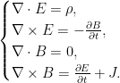
Here, ${E}$ is the electric field, ${B}$ is the magnetic field, ${\rho}$ is the charge density, and ${J}$ is the current density.
Continue reading “Maxwell’s equations” →

Tate’s thesis II – Global zeta functions

April 21, 2018April 21, 2018 Dongryul KimLeave a comment

In the previous post, we defined local zeta functions and meromorphically extended them to the complex plane. We now work towards defining the global zeta function. Although local zeta functions are supposed to be local factors of the zeta function, we are going to allow multiplying local zeta functions ${\zeta_v(f_v, c_v)}$ under some restrictive conditions. But let us first develop some general theory.

4. Fourier analysis on the adeles

We now start investigating the global analogue of the local theory we have developed so far. For ${K}$ a number field, we have different places ${v}$ and the corresponding completions ${K_v}$ , which are local fields.

Definition 1. We define the adeles ${\mathbb{A}_K}$ and the ideles ${\mathbb{A}_K^\times}$ as

$\displaystyle \begin{aligned} \mathbb{A}_K & \displaystyle= \{ (x_v)_v : x_v \in K_v, x_v \in \mathcal{O}_v \text{ for almost all } v \}, \\ \mathbb{A}_K^\times & \displaystyle= \{ (x_v)_v : x_v \in K_v^\times, x_v \in \mathcal{O}_v^\times \text{ for almost all } v \}, \end{aligned}$

with the topologies generated by, for ${S}$ finite, ${\prod_{v \in S}^{} U_v \times \prod_{v \notin S}^{} \mathcal{O}_v}$ in ${\mathbb{A}_K}$ and ${\prod_{v \in S}^{} U_v \times \prod_{v \notin S}^{} \mathcal{O}_v^\times}$ in ${\mathbb{A}_K^\times}$ . (Note that the topology of ${\mathbb{A}_K^\times}$ is not the subspace topology inherited from ${\mathbb{A}_K}$ .)

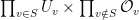
For all but finitely many places ${v}$ , the local field ${K_v}$ is going to be unramified over ${\mathbb{Q}_p}$ or ${\mathbb{F}_p}$ . This implies that ${\mathcal{D}_v = \mathcal{O}_v}$ for almost all ${v}$ . Then on ${\mathbb{A}_K}$ we may define the measure

$\displaystyle \mu\biggl( \prod_{v \in S}^{} U_v \times \prod_{v \notin S}^{} \mathcal{O}_v \biggr) = \prod_{v \in S}^{} \mu_v(U_v) \times \prod_{v \notin S}^{} \mu_v(\mathcal{O}_v)$

because for all but finitely ${v}$ , we have ${\mu_v(\mathcal{O}_v) = (N\mathcal{D}_v)^{-1/2} = 1}$ . We may further multiply all the local characters to get a character

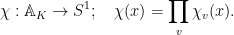
$\displaystyle \chi : \mathbb{A}_K \rightarrow S^1; \quad \chi(x) = \prod_{v}^{} \chi_v(x).$

This indeed is continuous because on the finite ${v}$ , the kernel contains ${\prod_{v \text{ fin}}^{} \mathcal{D}_v}$ and it is open. Continue reading “Tate’s thesis II – Global zeta functions” →

Tate’s thesis I – Local zeta functions

April 15, 2018April 15, 2018 Dongryul Kim1 Comment

The main goal of this series of posts is to give a brief summary of Tate’s thesis [Tat67]. Given a number field ${K}$ and a character ${\chi : \mathrm{Cl}_\mathfrak{m}(K) \rightarrow S^1}$ , one defines the Dirichlet ${L}$ -function as

$\displaystyle L(s, \chi) = \sum_{\mathfrak{a} \subseteq \mathcal{O}_K}^{} \frac{\chi(\mathfrak{a})}{(N\mathfrak{a})^s} = \prod_{\mathfrak{p} \subseteq \mathcal{O}_K}^{} \frac{1}{1 - (N\mathfrak{p})^{-s}},$

where we regard ${\chi(\mathfrak{a}) = 0}$ if ${(\mathfrak{a}, \mathfrak{m}) \neq 1}$ . Although this series converges only for ${\Re(s) > 1}$ , Hecke proved that the function extends meromorphically to the entire complex plane and moreover found a functional equation relating ${L(s, \chi)}$ and ${L(1-s, \overline{\chi})}$ . It turns out that we can define an analogous function for a character ${\chi : \mathbb{A}_K^\times / K^\times \rightarrow S^1}$ .

Tate’s contribution to this theory is to prove the functional equation and meromorphic extension in a systematic, elegant way. The main tool he uses is Fourier analysis on the adele ${\mathbb{A}_K}$ , in particular the Poisson summation formula. Because ${K}$ is discrete inside ${\mathbb{A}_K}$ with finite quotient, ${K}$ really can be thought of as a lattice inside ${\mathbb{A}_K}$ and the Poisson summation formula in this context can be written down. Imitating the proof of the functional equation for the Riemann zeta function in this context (with the right definition of the zeta function) then gives the functional equation.

The theory also gives new interpretations of classical knowledge on ${L}$ -functions. For example, the functional equation for the Riemann zeta function can be written as

$\displaystyle \pi^{-\frac{s}{2}} \Gamma\Bigl( \frac{s}{2} \Bigr) \zeta(s) = \pi^{-\frac{1-s}{2}} \Gamma\Bigl( \frac{1-s}{2} \Bigr) \zeta(1-s).$

Here, the additional factor

$\displaystyle \pi^{-\frac{s}{2}} \Gamma\Bigl( \frac{s}{2} \Bigr) = \int_{-\infty}^{\infty} e^{-\pi x^2} \lvert x \rvert^s \frac{dx}{\lvert x \rvert}$

can be interpreted as the contribution of infinity, so that the “completed” zeta function

$\displaystyle \xi(s) = \pi^{-\frac{s}{2}} \Gamma\Bigl( \frac{s}{2} \Bigr) \prod_{p}^{} \Bigl( 1 - \frac{1}{1 - p^{-s}} \Bigr)$

is the product of the local factors at each place, finite and infinite. The functional equation ${\xi(s) = \xi(1-s)}$ follows from a neat application of the Poisson summation formula in the adelic setting. Continue reading “Tate’s thesis I – Local zeta functions” →

Dwyer–Kan localization

March 20, 2018April 10, 2018 Dongryul Kim1 Comment

Classically, the localization ${\mathcal{C}[\mathcal{W}^{-1}]}$ of a (small) category ${\mathcal{C}}$ at a subcategory ${\mathcal{W}}$ is given by:

the objects of ${\mathcal{C}[\mathcal{W}]^{-1}}$ are objects of ${\mathcal{C}}$ ,
the morphisms ${\mathcal{C}[\mathcal{W}^{-1}](X, Y)}$ are diagrams
$\displaystyle X \rightarrow X_1 \xleftarrow{f_1} X_2 \rightarrow X_3 \leftarrow \cdots \rightarrow X_{2n-1} \xleftarrow{f_n} X_{2n} \rightarrow Y$

with ${f_i \in \mathcal{W}}$ , quotiented out by the obvious relations, and
composition is given by concatenation of diagrams.

This localization has the universal property that if ${F : \mathcal{C} \rightarrow \mathcal{D}}$ sends all morphisms of ${\mathcal{W}}$ to isomorphisms, then it factors uniquely through ${\mathcal{C} \rightarrow \mathcal{C}[\mathcal{W}^{-1}]}$ .

Our goal is to develop an analogue for ${(\infty,1)}$ -categories, using simplicial categories. Given a simplicial category ${\mathcal{C}}$ and a subcategory ${\mathcal{W}}$ , we would like to define a localization ${\mathcal{L}(\mathcal{C}, \mathcal{W})}$ , but we not only invert the arrows but also the “higher homotopy data” of arrows. The construction of simplicial localization was first given by Dwyer and Kan [DK80]. Continue reading “Dwyer–Kan localization” →

Faisceaux Algébriques Cohérents V – Serre duality

January 14, 2018January 14, 2018 Dongryul Kim2 Comments

Earlier, we have computed the dimension of ${H^i(\mathbb{P}_k^n, \mathscr{O}_X(m))}$ for all ${i}$ and ${m}$ . It turned out that it is ${0}$ for all ${i \neq 0, n}$ , and at ${i = 0, n}$ , we had

$\displaystyle \dim_k H^0(\mathbb{P}_k^n, \mathscr{O}_X(m)) \cong \dim_k H^n(\mathbb{P}_k^n, \mathscr{O}_X(-n-1-m)).$

This phenomenon is an instance of Serre duality. To explain this in detail, we first need to know a bit about ${\mathrm{Ext}}$ .

12. ${\mathrm{Ext}}$ and ${\mathscr{E}xt}$

We have define sheaf cohomology as the right derived functor of ${\Gamma(X,-)}$ . But we notice that this functor is isomorphic to ${\mathrm{Hom}_{\mathscr{O}_X}(\mathscr{O}_X, -)}$ . Also, ${\mathrm{Hom}}$ is left exact in general. This motivates us to define

Definition 1. Let ${(X, \mathscr{O}_X)}$ be a ringed space and ${\mathscr{F}}$ be an ${\mathscr{O}_X}$ -module. We define ${\mathrm{Ext}^i(\mathscr{F}, -)}$ as the right derived functors of ${\mathrm{Hom}(\mathscr{F}, -)}$ . Also, we define ${\mathscr{E}xt^i(\mathscr{F}, -)}$ as the right derived functors of ${\mathscr{H}om^i(\mathscr{F}, -)}$ .

From our motivation above, we immediately see that ${H^i(X, \mathscr{F}) \cong \mathrm{Ext}^i(\mathscr{O}_X, \mathscr{F})}$ . Here are some basic facts we will need.

Proposition 2 (Hartshorne III.6.8). Let ${(X, \mathscr{O}_X)}$ be a ringed space and ${\mathscr{F}, \mathscr{G} \in \mathsf{Mod}_{\mathscr{O}_X}}$ with ${\mathscr{F}}$ coherent. Then ${\mathscr{E}xt^i(\mathscr{F}, \mathscr{G})_x \cong \mathrm{Ext}^i_{\mathscr{O}_{X,x}}(\mathscr{F}_x, \mathscr{G}_x)}$ .

Proof. If we take an injective resolution ${0 \rightarrow \mathscr{G} \rightarrow \mathscr{J}^\bullet}$ , the left hand side is taking the sheaf hom ${\mathscr{H}om(\mathscr{F}, -)}$ and then taking stalks, while the right hand side is taking the stalk and taking ${\mathrm{Hom}(\mathscr{F}_x, -)}$ . Here, we note that ${\mathscr{J}}$ being an injective ${\mathscr{O}_X}$ -module implies that ${\mathscr{J}_x}$ is an injective ${\mathscr{O}_{X,x}}$ -module because we can look at skyscraper sheaves. So it suffices to show that ${\mathscr{H}om(\mathscr{F}, \mathscr{G})_x \cong \mathrm{Hom}_{\mathscr{O}_{X,x}}(\mathscr{F}_x, \mathscr{G}_x)}$ for any ${\mathscr{O}_X}$ -module ${\mathscr{G}}$ . To see this, we locally write ${\mathscr{O}_X^{m} \rightarrow \mathscr{O}_X^{n} \rightarrow \mathscr{F} \rightarrow 0}$ . Then

$\displaystyle 0 \rightarrow \mathscr{H}om(\mathscr{F}, \mathscr{G})_x \rightarrow \mathscr{H}om(\mathscr{O}_X^n, \mathscr{G})_x \rightarrow \mathscr{H}om(\mathscr{O}_X^m, \mathscr{G})_x$

and

$\displaystyle 0 \rightarrow \mathrm{Hom}_{\mathscr{O}_{X,x}}(\mathscr{F}_x, \mathscr{G}_x) \rightarrow \mathrm{Hom}_{\mathscr{O}_{X,x}}(\mathscr{O}_{X,x}^n, \mathscr{G}_x) \rightarrow \mathrm{Hom}_{\mathscr{O}_{X,x}}(\mathscr{O}_{X,x}^m, \mathscr{G}_x)$

shows what we want. ▨ Continue reading “Faisceaux Algébriques Cohérents V – Serre duality” →

Faisceaux Algébriques Cohérents IV – Coherent sheaves

January 13, 2018January 13, 2018 Dongryul Kim2 Comments

It’s quite awkward to be introducing coherent sheaves at this point, when the title of the paper is “Coherent algebraic sheaves”. So far, we’ve mostly gotten away with quasi-coherent sheaves. Serre introduces the notion of coherent sheaves, which contain some idea of finite generation in addition to being an quasi-coherent sheaf. But we want the class of sheaves to be form an abelian category. Finitely generated modules over a ring generally don’t form an abelian category, so we need an alternative notion.

11. Coherent sheaves

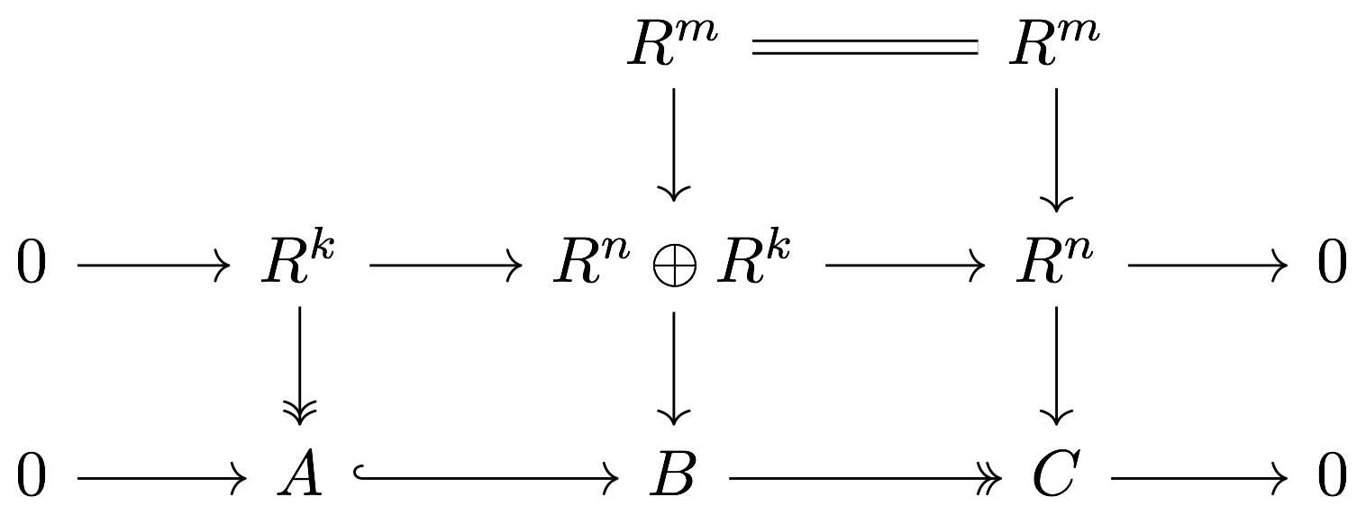
Definition 1. An ${R}$ -module is ${M}$ called finitely generated if there exists an integer ${n}$ with a surjection ${R^n \rightarrow M}$ . An ${R}$ -module ${M}$ is called coherent if it is finitely generated, and the cokernel of every (not necessarily surjective) map ${R^n \rightarrow M}$ is finitely generated.

This is equivalent to the seemingly weaker statement that every finitely generated submodule is finitely presented. If ${R}$ is Noetherian, a module is coherent if and only if it is finitely generated.

Proposition 2. If ${0 \rightarrow A \rightarrow B \rightarrow C \rightarrow 0}$ is a short exact sequence of ${R}$ -modules, and two of them is coherent, the last one is also coherent.

Proof. Suppose ${A}$ and ${B}$ are coherent. Because ${B}$ is finitely generated, ${C}$ is too. For an arbitrary map ${R^n \rightarrow C}$ , we can lift it to ${R^n \rightarrow B}$ . Also, there is a surjection ${R^k \rightarrow A}$ which induces ${R^k \rightarrow B}$ . Put them together to get a map ${R^n \oplus R^k \rightarrow B}$ , and continue it to an exact sequence ${R^m \rightarrow R^{n+k} \rightarrow B}$ using that ${B}$ is coherent. Then ${R^m \rightarrow R^n \rightarrow C}$ is exact after diagram chasing.

Continue reading “Faisceaux Algébriques Cohérents IV – Coherent sheaves” →

Faisceaux Algébriques Cohérents III – Coherent sheaves on projective space

January 12, 2018January 12, 2018 Dongryul KimLeave a comment

As we know, cohomology of sheaves on affine schemes is boring. The next simplest case we can consider is sheaves on projective schemes.

7. The ${\mathrm{Proj}}$ construction

We can define projective space by gluing affine space together, but there is a more canonical construction. By a graded ring ${S}$ , we implicitly assume that ${S = \bigoplus_{d \ge 0} S_d}$ .

Definition 1. The scheme ${\mathrm{Proj} S}$ is defined as the following. A point in ${\mathrm{Proj} S}$ is a homogeneous prime ideal ${\mathfrak{p}}$ of ${S}$ such that ${\mathfrak{p}}$ doesn’t contain all of ${S_1, S_2, \ldots}$ . The topology is generated by the sets ${D(f) = \{ \mathfrak{p} : f \notin \mathfrak{p}\}}$ for homogeneous ${f \in S_d}$ with ${d \ge 1}$ , and the structure sheaf on ${D(f)}$ is given by the ${\mathrm{Spec}}$ of the ${0}$ -th graded piece ${(S_f)_0}$ .

Example 1. If ${S = A[x_0, \ldots, x_n]}$ , we have ${\mathrm{Proj} S = \mathbb{P}_A^n}$ .

So any kind of section needs to come from a ${0}$ -th graded element in the ring. This makes sense, because on projective space, functions like ${x}$ or ${y^2 / (z+1)}$ don’t give well-defined values. On affine schemes, we were able to construct sheaves on ${\mathrm{Spec} A}$ from ${A}$ -modules. Similarly, we can construct sheaves on ${\mathrm{Proj} S}$ from graded ${S}$ -modules.

Definition 2. Let ${S}$ be a graded ring, and let ${M = \bigoplus_n M_n}$ be a graded ${S}$ -module. We define a quasi-coherent sheaf ${\tilde{M}}$ on ${\mathrm{Proj} S}$ , so that ${\tilde{M} \vert_{D(f)} \cong ((M_f)_0)^{\tilde{}}}$ .

The sheaves are glued via, where ${\deg f = a}$ and ${\deg g = b}$ , the isomorphisms ${((M_f)_0)_{g^a/f^b} \cong (M_{fg})_0 \cong ((M_g)_0)_{f^b / g^a}}$ . We immediately see that this is a quasi-coherent sheaf on ${\mathrm{Proj} S}$ . Of course, this construction is functorial in ${M}$ , and a short exact sequence ${0 \rightarrow M_1 \rightarrow M_2 \rightarrow M_3 \rightarrow 0}$ induces an exact sequence

$\displaystyle 0 \rightarrow \tilde{M}_1 \rightarrow \tilde{M}_2 \rightarrow \tilde{M}_3 \rightarrow 0$

of quasi-coherent sheaves, because the construction is exact affine-locally. Continue reading “Faisceaux Algébriques Cohérents III – Coherent sheaves on projective space” →